Lowering a distribution to a dynamical system

A delay distribution and a compartmental model are two views of the same thing. Gamma(3, 1.5) is a waiting time; it is also three exponential compartments in series, each left at rate 1/1.5. lower is the bridge: it maps a Distributions.Distribution onto a backend-agnostic dynamical-systems representation, which four package extensions then turn into the object a simulation or inference backend actually wants.

This page is the lowering itself; each backend then has its own page.

Lowering

Load the package and lower a few distributions.

using LoweredDistributions
using Distributions
using LinearAlgebra
using CairoMakie
using AlgebraOfGraphics
using DataFramesMeta

CairoMakie.activate!(type = "png", px_per_unit = 2)
set_theme!(theme_latexfonts(); fontsize = 14)

lower(Gamma(3.0, 1.5))

ErlangChain(3 compartments)

An Exponential is memoryless, so it lowers to a two-state continuous-time Markov chain (on -> absorbed) rather than a chain of compartments.

lower(Exponential(2.0))

CTMC continuous-time Markov chain
  states: on, absorbed
  on -> absorbed @ rate 0.5

A distribution with no exact chain representation is fitted by matching its first two moments: an under- or exactly-dispersed delay fits an ErlangChain, an over-dispersed one a branching (mixture) PhaseType. See phase_type for the full dispersion criterion.

lower(LogNormal(0.0, 0.5))      # c² ≈ 0.28 ≤ 1 -> ErlangChain

ErlangChain(4 compartments)

lower(Gamma(0.5, 1.0))          # c² = 2 > 1    -> PhaseType

PhaseType(2 phases)

Every phase-type representation converts to the canonical PhaseType(α, S) view: an initial distribution α over transient phases, and a sub-generator S whose row shortfalls are the exit rates to the absorbing state. This is the single shape each backend extension consumes, so the backend code does not care which fit produced it.

pt = PhaseType(lower(Gamma(3.0, 1.5)))

PhaseType(3 phases)

pt.S

3×3 Matrix{Float64}:
 -0.666667   0.666667   0.0
  0.0       -0.666667   0.666667
  0.0        0.0       -0.666667

Faithful lowering

Every backend reads the same PhaseType(α, S), so it is worth seeing directly how well that shape reproduces the distribution it came from. A phase-type's own density has a closed form, α' exp(S t) s, where s is the vector of per-phase exit rates (the row shortfalls of S), so it can be plotted against the exact density with no simulation at all.

function phasetype_density(pt::PhaseType, ts)
    s = -pt.S * ones(length(pt.α))
    return [only(transpose(pt.α) * exp(pt.S * t) * s) for t in ts]
end

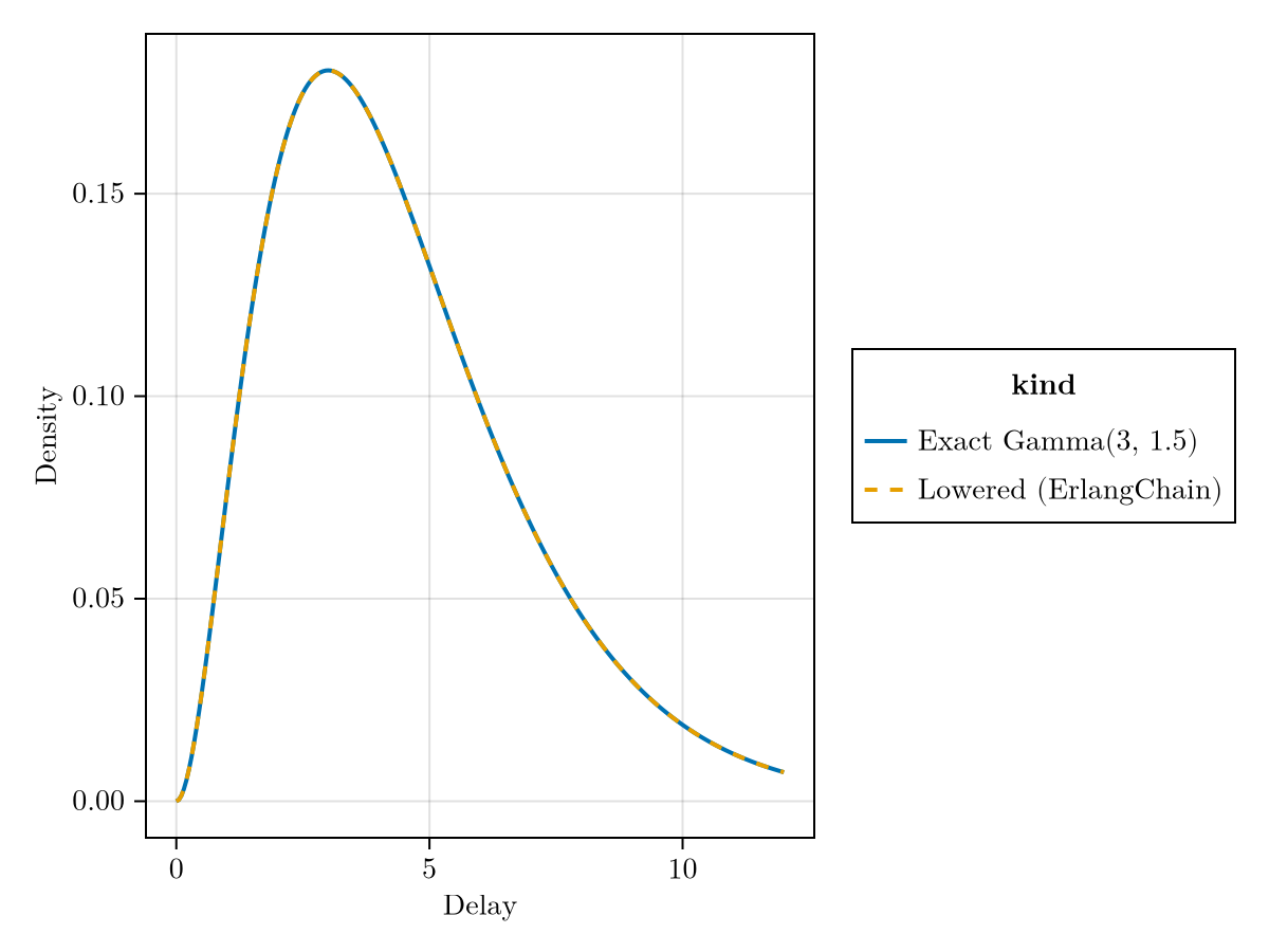
phasetype_density (generic function with 1 method)

Gamma(3, 1.5) has an integer shape, so its ErlangChain lowering is exact: the two curves sit on top of each other.

ts = 0.0:0.05:12.0
exact_df = DataFrame(t = collect(ts), density = pdf.(Gamma(3.0, 1.5), ts),
    kind = "Exact Gamma(3, 1.5)")
lowered_df = DataFrame(t = collect(ts), density = phasetype_density(pt, ts),
    kind = "Lowered (ErlangChain)")
draw(
    data(vcat(exact_df, lowered_df)) *
    mapping(:t, :density, color = :kind, linestyle = :kind) *
    visual(Lines, linewidth = 2);
    axis = (xlabel = "Delay", ylabel = "Density")
)

Gamma(0.5, 1.0) is over-dispersed (c² = 2), so it fits a branching PhaseType by matching only the first two moments, not the whole density. The exact density is singular at zero, which no finite phase-type can reproduce; away from that edge the moment-matched curve tracks the exact one reasonably, and the two share the same mean and variance by construction.

d_over = Gamma(0.5, 1.0)
pt_over = PhaseType(lower(d_over))
ts_over = 0.02:0.02:6.0
exact_over_df = DataFrame(t = collect(ts_over), density = pdf.(d_over, ts_over),
    kind = "Exact Gamma(0.5, 1.0)")
lowered_over_df = DataFrame(t = collect(ts_over),
    density = phasetype_density(pt_over, ts_over),
    kind = "Lowered (moment-matched PhaseType)")
draw(
    data(vcat(exact_over_df, lowered_over_df)) *
    mapping(:t, :density, color = :kind, linestyle = :kind) *
    visual(Lines, linewidth = 2);
    axis = (xlabel = "Delay", ylabel = "Density")
)

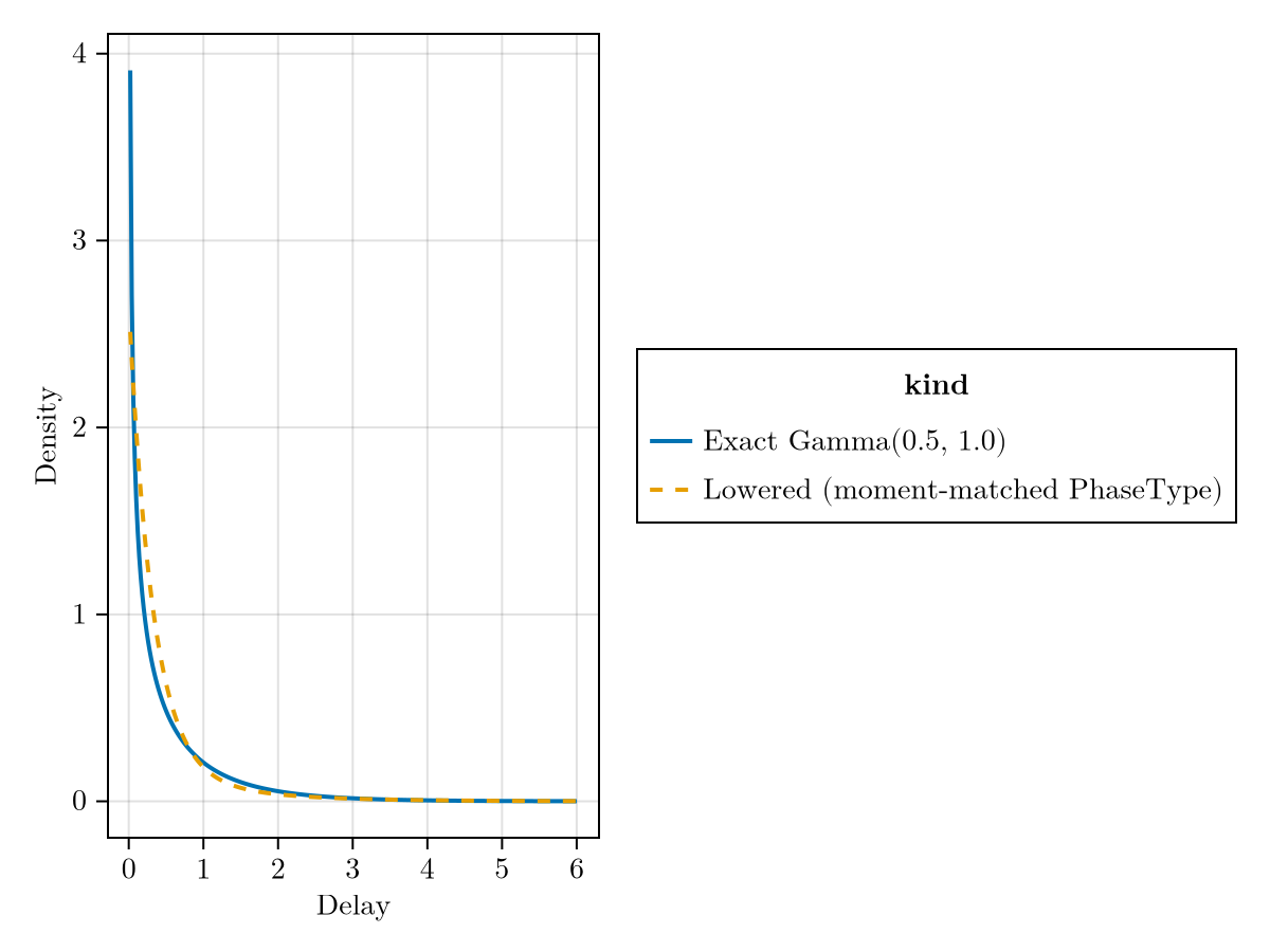
The two means agree exactly by construction; only an over-dispersed delay's shape is approximated.

mean(d_over), -sum(transpose(pt_over.α) * inv(Matrix(pt_over.S)))

(0.5, 0.5)

Which backend do I want?

Backend	Entry point	Gives you
SciMLBase	ode_problem	The linear forward-Kolmogorov ODE du/dt = Q'u: deterministic occupancy probabilities through time
Catalyst	reaction_system	A reaction network, so a lowered delay can be spliced onto a transition of a bigger model
JumpProcesses	jump_problem	Exact stochastic simulation (Gillespie/Doob) of one individual moving through the states
AlgebraicPetri	petri_net	A LabelledPetriNet, for composing models in the AlgebraicJulia ecosystem

Each backend page takes the same Gamma(3, 1.5) lowering and turns it into that backend's object, so the choice is about what you want to do with it, not about how the distribution was fitted.

Where next

• Public API for the full interface, including ctmc for building a chain by hand rather than by lowering a distribution.

• phase_type for the two-moment fit on its own, and compartment_stages for the raw (rate, stages) structure behind an ErlangChain.